Gradient Boost

Summary

Gradient boosting as another boosting algorithm used for machine learning. Similar to AdaBoost, this boosting technique relies on learning from previous decision trees. However, the key differences lie gradient boosting not using weak learners and having the same weighting attached to each tree.

This is gradient boosting for regression, meaning it will be a model for predicting a continues target.

---

Related Sections/Pre-Reading

• Classification Trees
• Random Forest
• AdaBoost
• Bias vs Variance

---

Content

The gradient boosting algorithm works by taking a base prediction, and then minimising the error of this prediction in order to get to a final value. This may sound confusing but I think it would be better to explain this in an example

The below example is using the following dataset, with the target being the price of the car. Dataset and example obtained from Link to Example

| Row Number	Cylinder Number	Car Height	Engine Location	Price
| 1	Four	48,8	Front	12000
| 2	Six	48,8	Back	16500
| 3	Five	52,4	Back	15500
| 4	Four	54,3	Front	14000

1. Creating Your Initial Prediction

Our initial prediction for the price of a new car will be quite simple and just be the average of the cars. Average = 14500.

We then insert this prediction into the above training data and calculate the residuals.Residuals relate to the error the prediction has from the actual data.

$\text{Residual}=\text{Observed Data}-\text{Predicted Data}$

Row Number	Cylinder Number	Car Height	Engine Location	Price	Prediction	Residual
1	Four	48,8	Front	12000	14500	-2500
2	Six	48,8	Back	16500	14500	2000
3	Five	52,4	Back	15500	14500	1000
4	Four	54,3	Front	14000	14500	-500

2. Creating a Model to Predict the Residual Amount

Now we will be using Decision Trees to predict the Residual Amount. This is key as we are not predicting the Price, which is the target value, but rather the error between our initial prediction and the observed data.

We will create the decision tree usingGiniImpurity . Please note that the tree’s created for gradient boosting will have a maximum fixed length decided on at the beginning of the project. This is to prevent too muchOverfitting in the data.

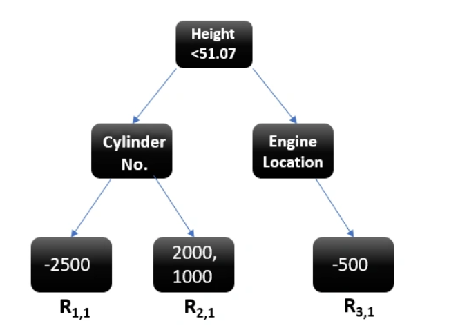
The following decision tree was created:

As you can see, there are some cases where we get more than 1 output per leaf (R2,1). We will replace these two values with a singular average for this leaf (1500)

Tree 1:

3. Update Predictions from Initial

This is the step where we go an update our prediction based off this new model we have created.

The updated prediction will look as following

$$\text{Prediction}=\text{Initial Prediction}+\text{Learning Rate}\times \text{Predicted Residual from Tree}$$

The learning rate is a multiple chosen between 0 and 1 at the start of the project. This is chosen to ensure that no single decision tree has too much bearing on the final project, reducing theOverfitting problem. We will use 0.1 for this example

For example, the new predicted value for Item 1 will be:

$$\text{Item 1 Prediction}=\text{Initial Prediction}+\text{Learning Rate}\times \text{Predicted Residual from Tree}$$ $$\text{Item 1 Prediction}=14500+(0.1\times 1500)$$ $$\text{Item 1 Prediction}=14650$$

Now we perform this prediction for all items in the table, calculate a list of all the new residual and again start from Step 2.

4. Conclusion

A fixed number of decision trees is decided upon at the beginning of the project and once that is reached, the full model will be ready to predict the data.

The hope is that as we continue along the decision trees, the residual amounts will decrease as we should be getting better at predicting the value